miércoles, 31 de octubre de 2012
martes, 30 de octubre de 2012
Programa 1: Análisis de respuesta y estabilidad de
Para esta semana la tarea de la materia de Automatización consiste en realizar un análisis en donde podemos ver cómo es la respuesta y estabilidad del sistema que hemos estado desarrollando durante el transcurso del semestre, por lo que voy a hacer un análisis en tiempo y frecuencia del circuito RLC en función de sus parámetros físicos utilizando el paquete de control de Octave.
Primero que nada, expongo el circuito RLC que hice en el modelo matemático.
En donde, sacamos una función de transferencia en la cual obtuvimos el siguiente resultado.
En donde como definimos, la L es la inductancia, R la resistencia y la C la capacitancia, por lo que podemos decir que esta función de transferencia está dada por sus parámetros físicos, pero para poder realizar el análisis en necesario tener las multiplicaciones de entrada y salida en función de s por lo que he multiplicado y agrupado para entender mejor el sistema.
Para tener como resultado una nueva función de transferencia equivalente a la anterior.
Esta sería la función de transferencia desde la entrada a voltaje de salida, por lo que podemos decir que en base a el libro de Ogata [1] de control moderno, para observar el comportamiento de nuestro circuito es necesario tener nuestro sistema en una frecuencia de 1 rad/s, por lo que podemos utilizar la inductancia y la capacitancia en un valor de uno y la variar resistencia del voltaje para saber como cámbia el sistema.
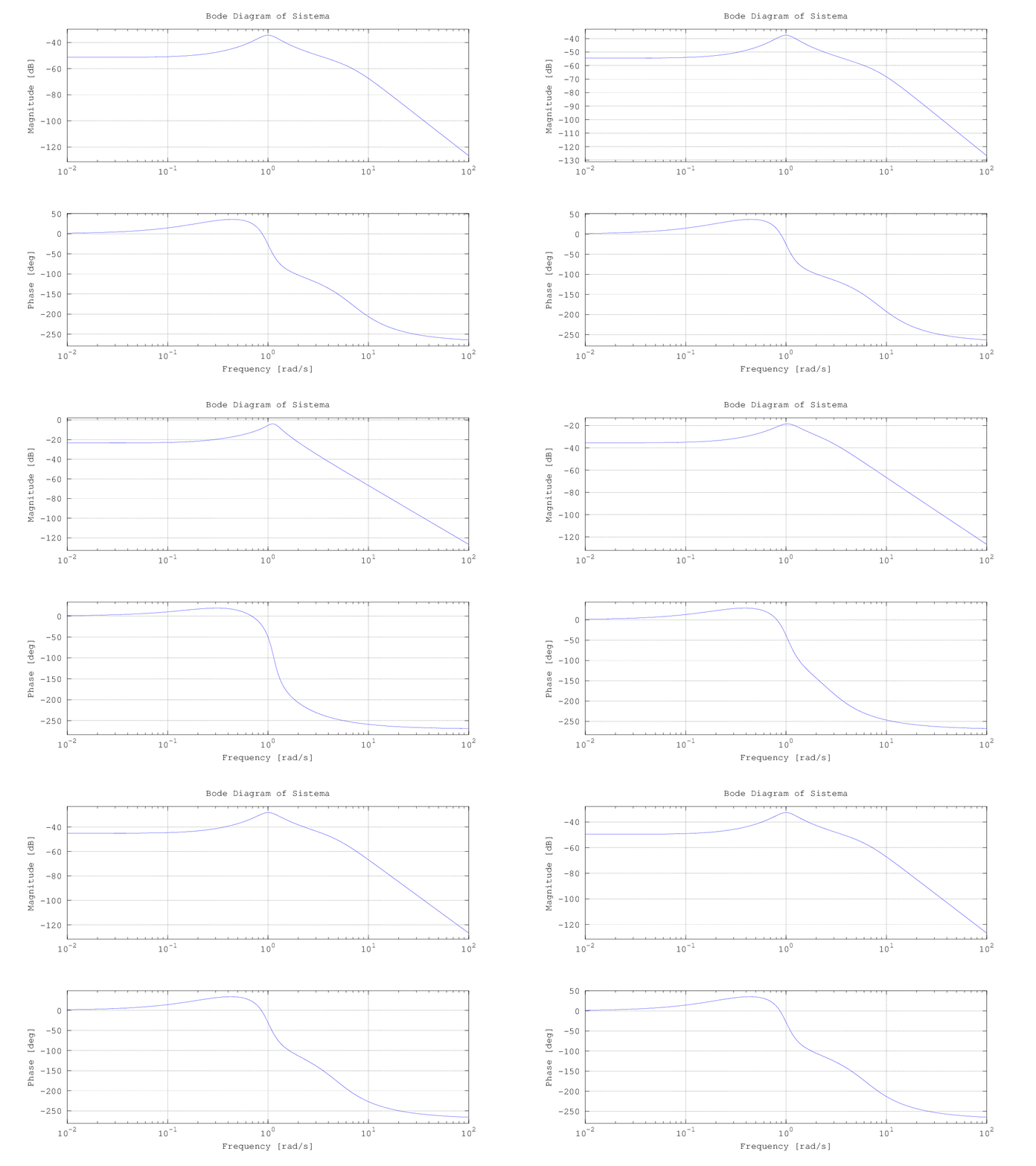
Entonces, para poder analizar la frecuencia de respuesta del circuito vamos a desarrollar una grafica Bode, herramienta que nos sirve de apoyo para investigar si el flujo de voltaje con características RLC esta generando una frecuencia estáble, por lo que primero tenemos que definir la función de transferencia e igualar los valores R, L, C en su valor minimo (En este caso puse un 1), para luego generar un diagrama bode en donde luego de estar variando la R, genero una pequeña animación para observar el comportamiento.
Podemos decir que respuesta en frecuencia es la respuesta del sistema que estamos observando en base a una entrada seno, por tanto, en el diagrama de bode podemos ver dos gráficas en donde en la parte superior vemos la representación en decibelios en contra una frecuencia logarítmica y en la parte inferior vemos los grados en contra una frecuencia logarítmica
Como definimos, tenemos un circuito RLC en donde tiene una ganancia máxima a frecuencia de 1 rad / s, en la parte media del de la representación de decibelios, pero vemos que la atenuación a nivel R = 2 ohms en frecuencia de 10 rad/s es de -60dB, luego en R = 14 ohms en frecuencia 10 rad/s es de -70dB, mientras que en R = 100 ohms tenemos una atenuación de -100dB, por lo que podemos decir que una R = 100 ohms podemos tener una ateniación más estrecha an base a la frecuencia de destino de 1 rad /s.
En base a [2], podemos decir que el punto crítico para medir la estabilidad de un sistema de control es el tener en un paso en la gráfica en -180 grados en la parte inferior y en la parte superior el paso de la linea en 0dB de manera que caigan de manera semejante, por lo que según mi punto de vista, este sistema no tiene una estabilidad ya que en la parte superior de magnitud nunca tenemos 0dB ni aunque la R = 1 menos en R = 100.
Ahora voy a realizar el análisis del tiempo de respuesta del circuito, en donde como podemos ver que en donde tenemos un mayor cambio de atenuación en el circuito es en R=15, vamos a sacar el análisis de tiempo en base a la función lsim() de octave la cual, calcula como evoluciona las salidas del sistema en conjunto con los estados de las entradas, es como si fuera una versión especial de step() en donde vemos los cambios, pero en cambio en lsim, estamos simulando el tiempo de respuesta producido de un sistema dinamico de control.
Las ondas nunca son atenuadas después o antes de 1 rad / seg, por lo que podemos decir que hemos tenido una respuesta no satisfactoria en base a el tiempo de respuesta, ya que si tuvieramos un sistema estable, veriamos una variación después de cierto tiempo, podemos ver que se generan gráficas de la misma magnitud.
Ahora les dejo el programa que hice para hacer estas gráficas y el análisis.
Por lo que podemos ver que en ninguno de los dos análisis que realizamos, obtuvimos resultados no satisfactorios, podemos concluir que mi sistema no es estable, considero, ahora que he estado leyendo sobre estabilidad y sobre lo que debería de hacer mi sistema, es que mi función de trasferencia está dada por factores físicos y por el sistema armónico, como lo describí en el modelado matemático, tal vez se necesite una forma de que el sistema armónico lo tengamos que poner en base a los factores físicos del RLC y tener así un sistema con una respuesta estable satisfactoria, ya que el sistema está siendo afectado directamente por las funciones trigonométricas que tengo de manera de salida.
Bibliografia.
[1] Chapter 3: Mathematical Modeling of Electrical Systems, Modern Control Engineering, Fifth Edition, Katsuhiko Ogata.
[2] Stability margins, models estim control, link
[3] Analyzing RLC Circuit, R2012b, link
Primero que nada, expongo el circuito RLC que hice en el modelo matemático.
En donde, sacamos una función de transferencia en la cual obtuvimos el siguiente resultado.
En donde como definimos, la L es la inductancia, R la resistencia y la C la capacitancia, por lo que podemos decir que esta función de transferencia está dada por sus parámetros físicos, pero para poder realizar el análisis en necesario tener las multiplicaciones de entrada y salida en función de s por lo que he multiplicado y agrupado para entender mejor el sistema.
Para tener como resultado una nueva función de transferencia equivalente a la anterior.
Esta sería la función de transferencia desde la entrada a voltaje de salida, por lo que podemos decir que en base a el libro de Ogata [1] de control moderno, para observar el comportamiento de nuestro circuito es necesario tener nuestro sistema en una frecuencia de 1 rad/s, por lo que podemos utilizar la inductancia y la capacitancia en un valor de uno y la variar resistencia del voltaje para saber como cámbia el sistema.
Entonces, para poder analizar la frecuencia de respuesta del circuito vamos a desarrollar una grafica Bode, herramienta que nos sirve de apoyo para investigar si el flujo de voltaje con características RLC esta generando una frecuencia estáble, por lo que primero tenemos que definir la función de transferencia e igualar los valores R, L, C en su valor minimo (En este caso puse un 1), para luego generar un diagrama bode en donde luego de estar variando la R, genero una pequeña animación para observar el comportamiento.
Podemos decir que respuesta en frecuencia es la respuesta del sistema que estamos observando en base a una entrada seno, por tanto, en el diagrama de bode podemos ver dos gráficas en donde en la parte superior vemos la representación en decibelios en contra una frecuencia logarítmica y en la parte inferior vemos los grados en contra una frecuencia logarítmica
![]() |
| Los valores R del 1 al 14 |
Podemos ver que hace cambios en frecuencia más drásticamente.
![]() |
| Los valores R del 15 al 100 |
Ahora, hace cambios de frecuencia menores en cada cambio de R.
Como definimos, tenemos un circuito RLC en donde tiene una ganancia máxima a frecuencia de 1 rad / s, en la parte media del de la representación de decibelios, pero vemos que la atenuación a nivel R = 2 ohms en frecuencia de 10 rad/s es de -60dB, luego en R = 14 ohms en frecuencia 10 rad/s es de -70dB, mientras que en R = 100 ohms tenemos una atenuación de -100dB, por lo que podemos decir que una R = 100 ohms podemos tener una ateniación más estrecha an base a la frecuencia de destino de 1 rad /s.
En base a [2], podemos decir que el punto crítico para medir la estabilidad de un sistema de control es el tener en un paso en la gráfica en -180 grados en la parte inferior y en la parte superior el paso de la linea en 0dB de manera que caigan de manera semejante, por lo que según mi punto de vista, este sistema no tiene una estabilidad ya que en la parte superior de magnitud nunca tenemos 0dB ni aunque la R = 1 menos en R = 100.
Ahora voy a realizar el análisis del tiempo de respuesta del circuito, en donde como podemos ver que en donde tenemos un mayor cambio de atenuación en el circuito es en R=15, vamos a sacar el análisis de tiempo en base a la función lsim() de octave la cual, calcula como evoluciona las salidas del sistema en conjunto con los estados de las entradas, es como si fuera una versión especial de step() en donde vemos los cambios, pero en cambio en lsim, estamos simulando el tiempo de respuesta producido de un sistema dinamico de control.
Las ondas nunca son atenuadas después o antes de 1 rad / seg, por lo que podemos decir que hemos tenido una respuesta no satisfactoria en base a el tiempo de respuesta, ya que si tuvieramos un sistema estable, veriamos una variación después de cierto tiempo, podemos ver que se generan gráficas de la misma magnitud.
Ahora les dejo el programa que hice para hacer estas gráficas y el análisis.
Por lo que podemos ver que en ninguno de los dos análisis que realizamos, obtuvimos resultados no satisfactorios, podemos concluir que mi sistema no es estable, considero, ahora que he estado leyendo sobre estabilidad y sobre lo que debería de hacer mi sistema, es que mi función de trasferencia está dada por factores físicos y por el sistema armónico, como lo describí en el modelado matemático, tal vez se necesite una forma de que el sistema armónico lo tengamos que poner en base a los factores físicos del RLC y tener así un sistema con una respuesta estable satisfactoria, ya que el sistema está siendo afectado directamente por las funciones trigonométricas que tengo de manera de salida.
Bibliografia.
[1] Chapter 3: Mathematical Modeling of Electrical Systems, Modern Control Engineering, Fifth Edition, Katsuhiko Ogata.
[2] Stability margins, models estim control, link
[3] Analyzing RLC Circuit, R2012b, link
Tarea 9: Grafo de programa
Para esta entrada de verificación voy a hacer un sistema en donde podamos modelar en base al reciclaje del papel, por lo que podemos decir que el sistema consta de los siguientes procesos.
Ahora, en base a estos procedimiento, voy a crear el sistema en base al estado del papel en donde según el estado, vamos a crear las transiciones del sistema dado el siguiente diagrama.
En donde el sistema global inicial es 0000, pero para poder iniciar el ciclo necesitamos por lo menos tener papel, por lo que pongo como estado global el tener papel recolectado 1000.
Bibliografia.
Principles of Model Cheking, Baier & Katoen,
- Recolectar papel y Clasificar el papel(Recolección)
- Se moja y se bate para crear pasta (Creación_pasta)
- Se limpia la pasta de pegamento, tintes, etc. (Limpieza)
- Se moldea en superficia plana. (Molde_pasta)
- Secado y enrollado de hoja. (Generar_papel)
Ahora, en base a estos procedimiento, voy a crear el sistema en base al estado del papel en donde según el estado, vamos a crear las transiciones del sistema dado el siguiente diagrama.
En donde el sistema global inicial es 0000, pero para poder iniciar el ciclo necesitamos por lo menos tener papel, por lo que pongo como estado global el tener papel recolectado 1000.
Bibliografia.
Principles of Model Cheking, Baier & Katoen,
Etiquetas:
Verificación y validación de software
miércoles, 24 de octubre de 2012
Stream Cipher: E0
Hi! for this week we need to choose a stream cipher to investigate and also put an example, so, I chose E0 which is the algorithm that is used to protect the confidentiality of communication protocol in wireless Bluetooth, developed by Bluetooth Special Interest Group (SIG) [1] including 1500 companies.
The pseudo-random generator consists with four LFSRs (Linear feedback shift register) combined by a function having 4 bits of internal memory which is updated by a nonlinear function. Bluetooth work on the principle of a protocol for master-slave type.
Vulnerability: E0 is vulnerable with the fast correlation attack that can recover the encrypthon key in 2^38 operations if we know the first 24 bits.
If we need to implement a security using E0 must have the following parameters.
Under the bluetooth protocol, data is transmitted in the form of frames more than 2745 bits, so, each frame is encrypted by modulo 2 bit by bit with the first output bit of the pseudo-random generatos, initialized with a secret key which is the same during the session and an initial value which is modified at each frame change.
Description
E0 uses a combination of four LFSRs[5], and having a 4 bits in memory, this is used at two different levels, it is applied once furing initialization to generate an initial state of 128 bits from the secret key and the first vector and the same mechanism is then used to produce the keystream from this initial state[4].
The four registers LFSRs are binary with this lengths L1 = 25, L2= 31, L3=33, L4 = 39, total = 128 bits.
If we denote xit the output at time t with i-th LFSR, then we need to calculate the 3-bit integer (0 to 4) corresponding to the sum of the outputs of the four LFSRs.
We need a combiner function F, that is a 4-bit finite state machine, if we have ct =(qt , pt , qt-1, pt-1) it's the registers of F and l(t) = x1t+ x2t+ x3t+ x4t is integer addition.
The output of the combiner function is pt, so, pt = F(xt, ct)
The state change by the following instruction:
where
St+1is the binary representation of the right number, 1 most significant bit and 0 least significant bit.
The output of the algorithm is:
So, we can say that the E0 algorithm made for each packet transmissions generates a new encryption that combine the four registers (complex RAND, device address, master clock, secret key), which has a 25, 31, 33, 39 bits, 128 in total, the secret key is used as an input to E0 to produce a bit stream pt that is added with modulo 2 to be encrypted.
Example
So, this is my example, I use for made the calculation, python in console mode.
We need 4 variables, with determinate bits:
RAND = 1101101000001010110100111 (25 bits)
Device Address = 1101111001010011010001010100011 (31 bits)
Master Clock = 111000001001110111101000111001001 (33 bits)
Secret Key =110010111000000010100110010100110001101 (39 bits)
I just use random numbers generates with the function getrandbits in python, then, we need to do LFRS, so this is one iteration, we need to select the position base on the polynomials and made the sum.
P1(x) = 1 + 0 + 0 + 1 + 1
P1(x) = 11
P2(x) = 1 + 0 + 0 + 0 + 1
P2(x) = 10
P3(x) = 1 + 0 + 0 + 1 + 1
P3(x) = 11
P4(x) = 1 + 1 + 1 + 0 + 1
P4(x) = 100
Then, we need to have lt
lt = 11 + 10 + 11 + 100
lt = 1100
Then we need to calcule F(xt, ct) if we have ct =(qt , pt , qt-1, pt-1) as memory of previous iterations, base in [1] we have 2 states 2-bit that:
Suppose that we have this combination and a t = 35 seg:
qt = 00
pt = 01
qt-1 = 11
pt-1= 10
St+1= floor(pi(100011)+2*(00)+01/2)
St+1 = 11110
pt = F(xt, ct)
pt = 11110
Then we can calculate Z:
Z = (l(t) % 2) + Pt
Z = (1100 % 2) + 11110
Z = 11110
So, Z contains one bit stream encrypted, this change in the time and in the state.
Vulnerability
The generator by combining registers used in the algorithm e0 is vulnerable to several attacks, I can mention for example linear attack, algebraic and fast algebraic attacks and fast correlation attacks. Most of these attacks requires the knowledge of a large number of successive bits of the key, which is not possible in the practical context of the Bluetooth protocol since the initial state of the generator is changed every number of bits.
By cons, sophisticated correlation attacks, presented by Yi Lu, Wili Meier [2], take into the session the re-synchronization occurs after encrypting each frame, and also there are one most effective[3] that allows to recover the encryption key from the knowledge of the first 24 bits of 2223.8 frames in 238 operations, as a result, the algorithm used in Bluetooth e0 is clearly offers insufficient security.
Biography.
[1] Bluetooth special interest group link
[2] Cryptanalysis of Bluetooth Keystream Generator Two-Level E0, Yi Lu, link
[3] A Practical Arrak on Bluetooth Encryption, Vili Meier, link
[4] Criptografía Moderana, cifra de flujo, P. Caballero link
[5] Communication Systems Security, Appendix B.L. Chen, link
[6] Algebraic Attacks and Stream Ciphers, Mikko Kiviharju, link

The pseudo-random generator consists with four LFSRs (Linear feedback shift register) combined by a function having 4 bits of internal memory which is updated by a nonlinear function. Bluetooth work on the principle of a protocol for master-slave type.
If we need to implement a security using E0 must have the following parameters.
- Key length: 128 bits, the key is always extended to a word of 128 bits by adding bits redundancy even when the actual number of bits is less key.
- Initialization 64 bits vector, corresponding to the logical address of the master (48 bits) and the data of the clock (22 bits).
Under the bluetooth protocol, data is transmitted in the form of frames more than 2745 bits, so, each frame is encrypted by modulo 2 bit by bit with the first output bit of the pseudo-random generatos, initialized with a secret key which is the same during the session and an initial value which is modified at each frame change.
Description
![]() |
| E0 diagram[6] |
E0 uses a combination of four LFSRs[5], and having a 4 bits in memory, this is used at two different levels, it is applied once furing initialization to generate an initial state of 128 bits from the secret key and the first vector and the same mechanism is then used to produce the keystream from this initial state[4].
The four registers LFSRs are binary with this lengths L1 = 25, L2= 31, L3=33, L4 = 39, total = 128 bits.
If we denote xit the output at time t with i-th LFSR, then we need to calculate the 3-bit integer (0 to 4) corresponding to the sum of the outputs of the four LFSRs.
The output of the combiner function is pt, so, pt = F(xt, ct)
The state change by the following instruction:
where
St+1is the binary representation of the right number, 1 most significant bit and 0 least significant bit.
The output of the algorithm is:
So, we can say that the E0 algorithm made for each packet transmissions generates a new encryption that combine the four registers (complex RAND, device address, master clock, secret key), which has a 25, 31, 33, 39 bits, 128 in total, the secret key is used as an input to E0 to produce a bit stream pt that is added with modulo 2 to be encrypted.
Example
So, this is my example, I use for made the calculation, python in console mode.
We need 4 variables, with determinate bits:
RAND = 1101101000001010110100111 (25 bits)
Device Address = 1101111001010011010001010100011 (31 bits)
Master Clock = 111000001001110111101000111001001 (33 bits)
Secret Key =110010111000000010100110010100110001101 (39 bits)
I just use random numbers generates with the function getrandbits in python, then, we need to do LFRS, so this is one iteration, we need to select the position base on the polynomials and made the sum.
P1(x) = 1 + 0 + 0 + 1 + 1
P1(x) = 11
P2(x) = 1 + 0 + 0 + 0 + 1
P2(x) = 10
P3(x) = 1 + 0 + 0 + 1 + 1
P3(x) = 11
P4(x) = 1 + 1 + 1 + 0 + 1
P4(x) = 100
Then, we need to have lt
lt = 11 + 10 + 11 + 100
lt = 1100
Then we need to calcule F(xt, ct) if we have ct =(qt , pt , qt-1, pt-1) as memory of previous iterations, base in [1] we have 2 states 2-bit that:
Suppose that we have this combination and a t = 35 seg:
qt = 00
pt = 01
qt-1 = 11
pt-1= 10
St+1= floor(pi(100011)+2*(00)+01/2)
St+1 = 11110
pt = F(xt, ct)
pt = 11110
Then we can calculate Z:
Z = (l(t) % 2) + Pt
Z = (1100 % 2) + 11110
Z = 11110
So, Z contains one bit stream encrypted, this change in the time and in the state.
Vulnerability
The generator by combining registers used in the algorithm e0 is vulnerable to several attacks, I can mention for example linear attack, algebraic and fast algebraic attacks and fast correlation attacks. Most of these attacks requires the knowledge of a large number of successive bits of the key, which is not possible in the practical context of the Bluetooth protocol since the initial state of the generator is changed every number of bits.
By cons, sophisticated correlation attacks, presented by Yi Lu, Wili Meier [2], take into the session the re-synchronization occurs after encrypting each frame, and also there are one most effective[3] that allows to recover the encryption key from the knowledge of the first 24 bits of 2223.8 frames in 238 operations, as a result, the algorithm used in Bluetooth e0 is clearly offers insufficient security.
Biography.
[1] Bluetooth special interest group link
[2] Cryptanalysis of Bluetooth Keystream Generator Two-Level E0, Yi Lu, link
[3] A Practical Arrak on Bluetooth Encryption, Vili Meier, link
[4] Criptografía Moderana, cifra de flujo, P. Caballero link
[5] Communication Systems Security, Appendix B.L. Chen, link
[6] Algebraic Attacks and Stream Ciphers, Mikko Kiviharju, link
Suscribirse a:
Entradas (Atom)


+22.42.57.png)

+15.52.34.png)


+16.19.55.png)